
MY NUMBER 1 RECOMMENDATION TO CREATE FULL TIME INCOME ONLINE: CLICK HERE
Microsoft Excel allows you to do more than simply create spreadsheets – you can also use the software to calculate key functions such as the ratio of two variables. This metric, known as the correlation coefficient, is useful for measuring the impact of one operation on another to inform business operations.
Not confident in your Excel skills? WIthout problems. Here’s how to calculate—and understand—the correlation coefficient in Excel.
![Download 10 Excel Templates for Marketers [Free Kit]](https://no-cache.hubspot.com/cta/default/53/9ff7a4fe-5293-496c-acca-566bc6e73f42.png)
What is correlation?
Correlation measures the relationship between two variables. A correlation coefficient of 0 means that the variables have no effect on each other – increases or decreases in one variable have no consistent effect on the other.
A correlation coefficient of +1 indicates “perfect positive correlation,” meaning that as variable X increases, variable Y increases at the same rate. A correlation value of -1, meanwhile, is “perfect negative correlation,” meaning that as variable X increases, variable Y decreases at the same rate. Correlation analysis can also return results anywhere between -1 and +1, meaning that the variables change at similar but not identical rates.
Correlation values can help companies assess the impact of certain actions on other actions. For example, companies can identify this as spending on social media marketing increases, as well customer engagementsuggesting that spending more might make sense.
However, they may find that certain campaigns result in a correlated decrease in customer engagement, suggesting a need to reevaluate current efforts. Finding that variables are uncorrelated can also be valuable; while common sense may suggest that a new feature or feature in your product would correspond to greater engagement, it may not have a measurable impact. Correlation analysis allows companies to look at this relationship (or lack thereof) and make good strategic decisions.
How to Calculate Correlation Coefficient in Excel
- Open Excel.
- Install the Analysis Toolpak.
- Select “Data” from the top bar menu.
- Select “Data Analysis” in the upper right corner.
- Select Correlation.
- Specify the data range and output.
- Estimate your correlation coefficient.
So how do you calculate the correction factor in Excel? Simple! Follow these steps:
1. Open Excel.
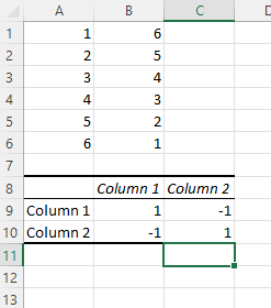
Step One: Open Excel and start a new worksheet for the correlated variables data. Enter the data points of your first variable in column A and your other variables in column B. You can also add additional variables in columns C, D, E, etc. — Excel will provide a correlation coefficient for each.
In the example below, we entered six rows of data into column A and six into column B.

2. Install Analysis Toolpak.
Next? If you don’t have one, install the Excel Analysis Toolpak.
Select “File” and then “Options” and you will see this screen:

Select “Add-ons” and then click “Go.”
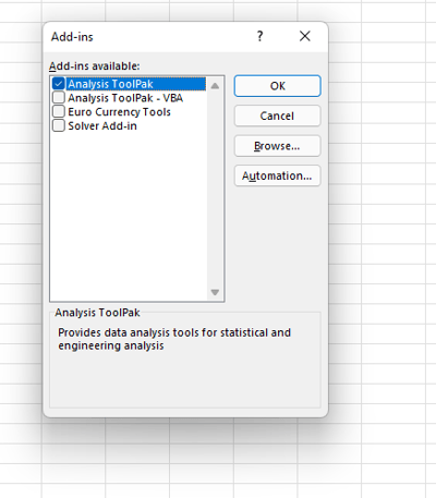
Now check the box that says “Analysis ToolPak” and click “OK”.
3. Select “Data” from the top bar menu.
After installing the ToolPak, select “Data” from the top menu of the Excel bar. This provides you with a sub-menu containing various options for analyzing your data.
4. Select “Data Analysis” in the upper right corner.
Now find “Data Analysis” in the upper right corner and click on it to get this screen:
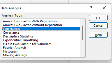
5. Select Correlation.
Select Correlation from the menu and click OK.
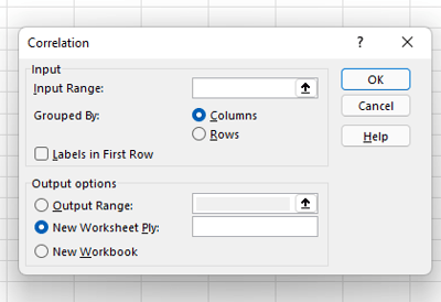
6. Define data scope and output.
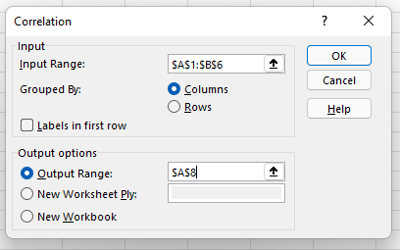
Now define the data range and output. You can simply left-click and drag your cursor over the data you want to select and it will automatically be entered into the Correlation box. Finally, choose an output range for your correlation data – we chose A8. Then click “OK”.
7. Estimate your correlation coefficient.
Your correlation results will now be displayed. In our example, the values in column 1 and column 2 have a perfect negative correlation; as one rises, the other descends at the same rate.
Excel correlation matrix
Excel correlation results are also known as Excel correlation matrix. In the example above, our two columns of data created a complete correction matrix of 1 and -1. But what happens if we construct a correlation matrix with a less-than-ideal data set?
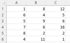
Here are our details:
And here is the matrix:
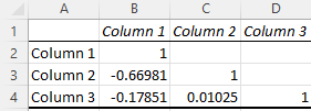
Cell C4 in the matrix gives us a correlation between column 3 and column 2 which is a very weak 0.01025, while column 1 and column 3 give a stronger negative correlation of -0.17851. By far the strongest correlation is between column 1 and column 2 at -0.66891.
So what does this mean in practice? Let’s say we were studying the impact of certain actions on the effectiveness of a social media campaign, where column 1 represents the number of visitors who click on social media ads, and columns 2 and 3 represent two different marketing slogans. The correlation matrix shows a strong negative correlation between columns 1 and 2, indicating that the tagline version in column 2 significantly decreased overall user engagement, while column 3 caused only a slight decrease.
Regularly creating Excel matrices can help companies better understand the impact of one variable on another and identify what (if any) negative or positive effects there may be.
Excel correlation formula
If you want to enter the correlation formula yourself, that is also an option. It looks like this:
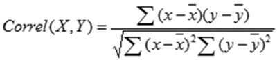
X and Y are your measurements, ∑ is the sum, and X and Y with lines above them indicate the mean of the measurements. It would be calculated as follows:
- Calculate the sum of variable X minus the mean of X.
- Calculate the sum of the variable Y minus the mean of Y.
- Multiply these two results and set this number aside (this is the first result).
- Square the sum of X minus the mean of X. Square the sum of Y minus the mean of Y. Multiply these two numbers.
- Extract the square root (this is the second result).
- Divide the first result by the second result.
- You get the correlation coefficient.
Simple, right? Yes and no. While inserting numbers isn’t complicated, creating and managing this formula is often more trouble than it’s worth. The built-in Excel Toolpak is often an easier (and faster) way to accurately determine coefficients and discover key relationships.
Correlation ≠ Not causation
No article on correlation is complete without mentioning that it is not the same as causation. In other words, just because two variables increase or decrease together does not mean that one variable is the cause of the increase or decrease in the other variable.
Consider some very unusual cases.

This figure shows an almost perfect negative correlation between the number of pirates and the global average temperature – when there were fewer pirates, the average temperature rose.
The problem? Although these two variables are related, there is no causal relationship between them; higher temperatures did not reduce pirate populations and fewer pirates did not cause global warming.
While correlation is a powerful tool, it only shows the direction of increase or decrease between two variables—not the cause of that increase or decrease. To discover causal relationships, companies must increase or decrease one variable and observe the impact. For example, if the correlation shows that customer engagement increases with social media spending, it is worth choosing to increase spending slightly, followed by measuring the results. If higher spending leads directly to higher engagement, the connection is both correlated and causal. If not, there may be one (or more) factors supporting an increase in both variables.
Keeping up with the correlations
Excel correlations provide a solid starting point for developing marketing, sales and spending strategies, but they don’t tell the whole story. Therefore, it is worth using Excel’s built-in data analysis options to quickly evaluate the correlation between two variables and use this data as a starting point for more in-depth analysis.

MY NUMBER 1 RECOMMENDATION TO CREATE FULL TIME INCOME ONLINE: CLICK HERE